Results are collected, optimised, and processed multiple times per day. Instagram images tagged with #hottest100 and a few others are included for counting.
It’s been a long time since the Hottest 100 of 2016 was aired. Unfortunately, I never really got around to publishing some analysis I performed on the prediction results. Fortunately, I managed to find some time recently!
Looking from afar, the results don’t look fantastic (when you compare them to my results from 2015 at least). The prediction unfortunately predicted the top two places out of order, however did manage to predict the third place correctly.
Lets take a look at the Top 10 of Triple J’s list and match it up with 100 Warm Tunas:
Looking at this we see most predictions we can find some learnings:
The average error for the top ten rank was 1.9 rank positions.
If 100 Warm Tunas ignored rank and simply guessed the top ten, it would have predicted 8 of the top 10 songs.
If 100 Warm Tunas ignored rank and simply guessed the top 3 songs to win, it would have predicted all 3 songs. Woo!
Lets dive into a chart that shows error for all ranks:
From this chart, we can deduce that the further away from position 1 we become, the higher the error. This information alone isn’t very useful. We can get a better understanding of error by finding the average for each ranking group:
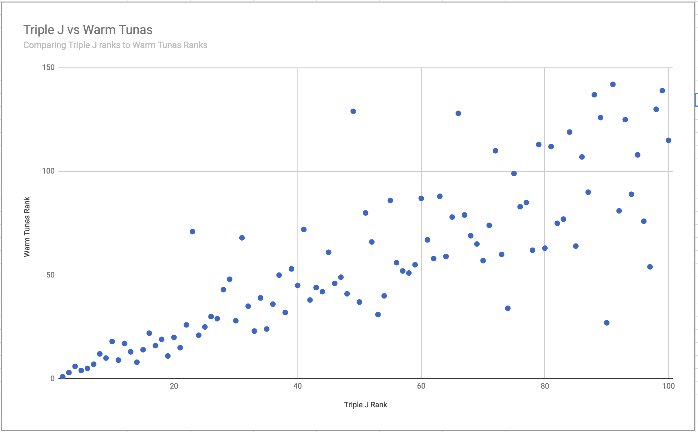
As we get closer to rank 1, the results become more and more accurate, however they are not perfect. This is more obvious if we use a scatter plot to compare Triple J ranks against Warm Tunas predictions:
It’s clear now that as we get closer to rank 1, the 100 Warm Tunas prediction gets better and converges upon the actual rankings played out on the day. However, unfortunately this year the difference between rank 1 and rank 2 was way too close to call - just 0.67% of voting volume was separating the two. A difference that was not enough to provide an accurate prediction of the winner.
Overall, whilst 100 Warm Tunas 2016 did get the two top positions out of order, it’s understandable as to why this happened. Hopefully this year there is a greater difference between ranks, giving further ability to predict the winner in position #1.
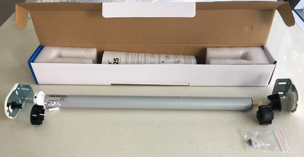
I’ve been doing a fair bit of DIY home automation hacking lately across many different devices - mostly interested in adding DIY homekit integrations. A couple of months ago, my dad purchased a bulk order of RAEX 433MHz RF motorised blinds to install around the house, replacing our existing manual roller blinds.
Note: If you are based in Australia, you can purchase these in bulk or individually via www.raexaustralia.com (Full disclosure – my father runs the site).
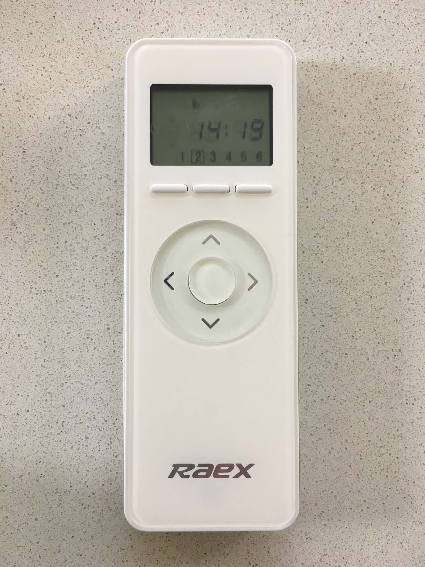
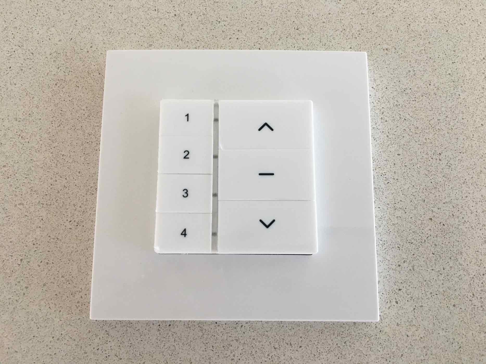
The blinds are a fantastic addition to the house, and allow me to be super lazy opening/closing my windows, however in order to control them you need to purchase the RAEX brand remotes. RAEX manufacture many different types of remotes, of which, I have access to two of the types, depicted below:
R Type Remote (YRL2016)
X Type Remote (YR3144)
Having a remote in every room of the house isn’t feasible, since many channels would be unused on these remotes and thus a waste of $$$ purchasing all the remotes. Instead, multiple rooms are programmed onto the same remote. Unfortunately due to this, remotes are highly contended for.
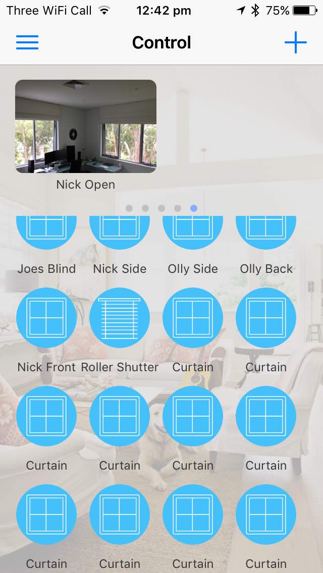
An alternate solution to using the RAEX remotes is to use a piece of hardware called the RM Pro. This allows you to control the remotes via your smartphone using their app
The app is slow, buggy and for me, doesn’t fit well into the home-automation ecosystem. I want my roller blinds to be accessible via Apple Homekit.
In order to control these blinds, I knew I’d need to either:
Reverse engineer how the RM Pro App communicated with the RM Pro and piggy-back onto this
Reverse engineer the RF protocol the remotes used to communicate with the blinds.
I attempted option 1 for a little while, but ruled it out as I was unable to intercept the traffic used to communicate between the iPhone and the hub. Therefore, I began my adventure to reverse engineer the RF protocol.
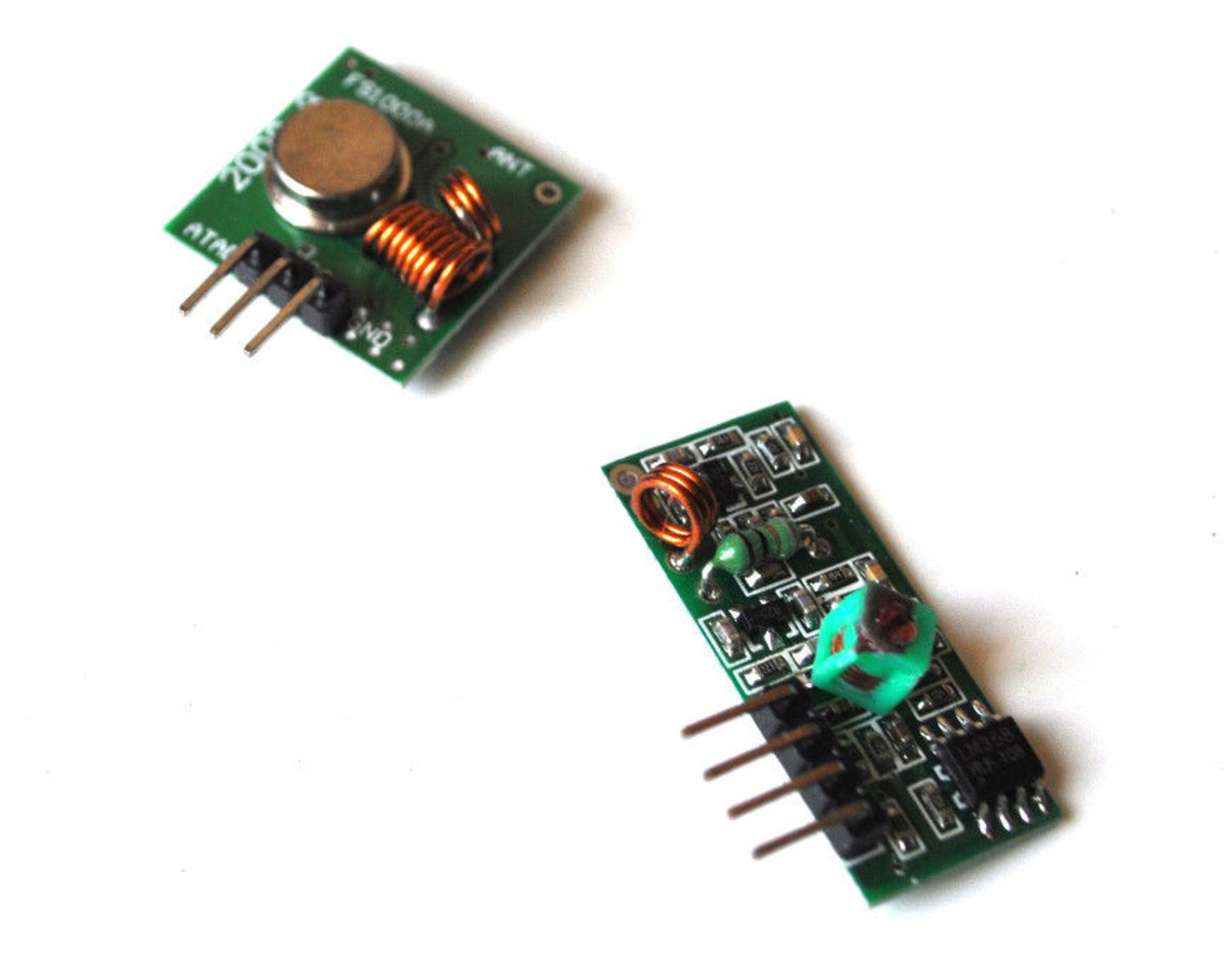
I purchased a 433MHz transmitter/receiver pair for Arduino on Ebay. In case that link stops working, try searching Ebay for 433Mhz RF transmitter receiver link kit for Arduino.
Initial Research
A handful of Google searches didn’t yield many results for finding a technical specification of the protocol RAEX were using.
I could not find any technical specification of the protocol via FCC or patent lookup
Emailed RM Pro to obtain technical specification; they did not understand my English.
Emailed RAEX to obtain technical specification; they would not release without confidentiality agreement.
I did find that RFXTRX was able to control the blind via their BlindsT4 mode, which appears to also work for Outlook Motion Blinds.
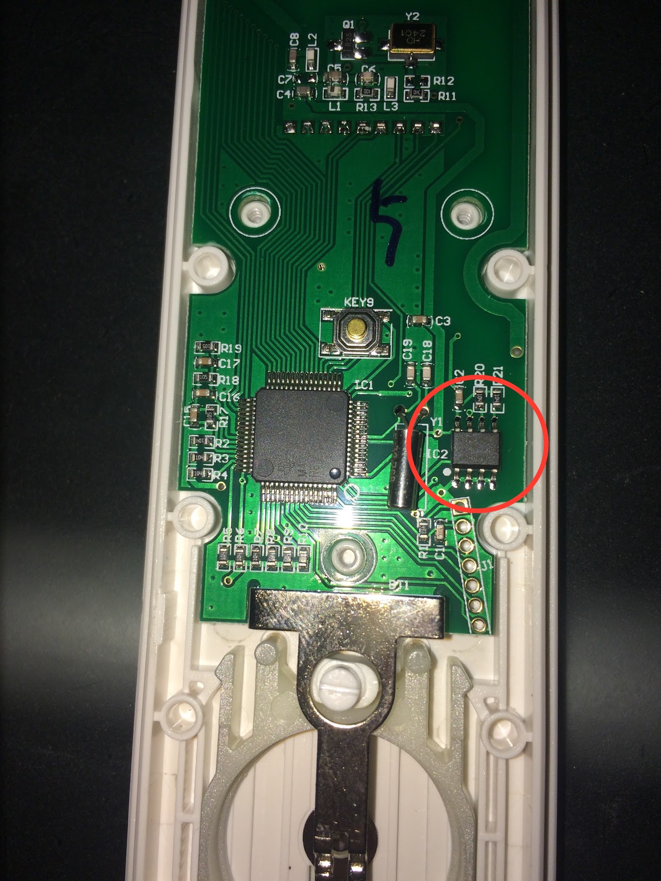
After opening one of the remotes and identifying the micro-controllers in use, I was unable to find any documentation explaining a generic RF encoding scheme being used.
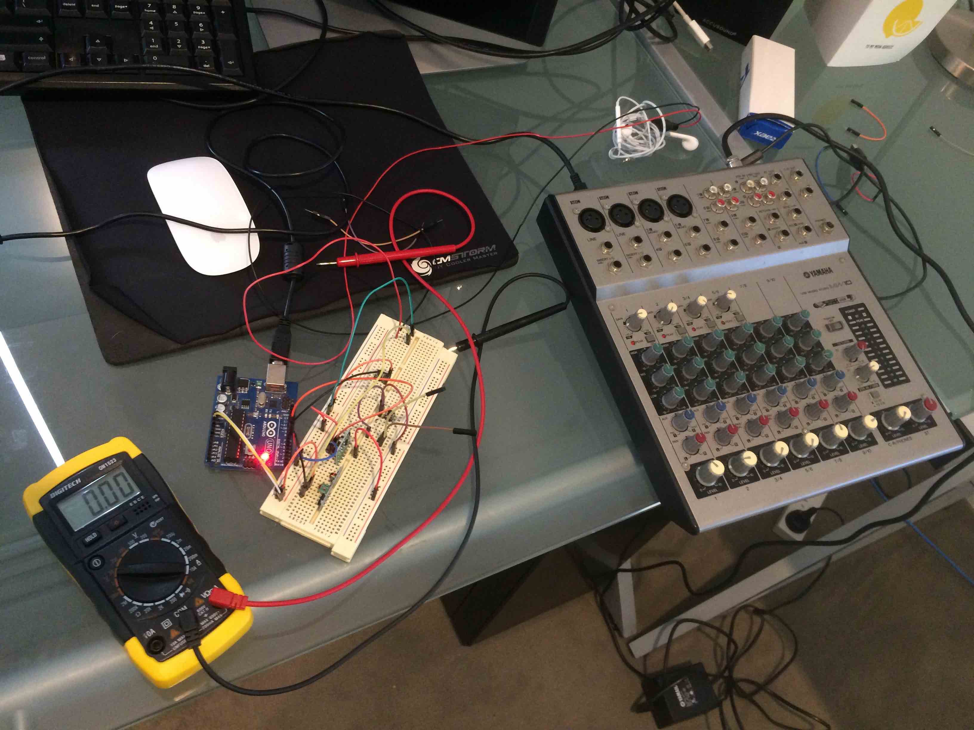
Once my package had arrived I hooked up the receiver to an Arduino and began searching for an Arduino sketch that could capture the data being transmitted. I tried many things that all failed, however eventually found one that appeared to capture the data.
Once I captured what I deemed to be enough data, I began analysing it. It was really difficult to make any sense of this data, and I didn’t even know if what had been captured was correct.
I did somefurtherreading and read a few RF reverse engineering write-ups. A lot of them experimented with the idea of using Audacity to capture the signal via the receiver plugged into the microphone port of the computer. I thought, why not, and began working on this.
This captures a lot of data. I captured 4 different R type remotes, along with 2 different X type remotes, and to make things even more fun, 8 different devices pairings from the Broadlink RM Pro (B type).
From this, I was able to determine a few things
The transmissions did not have a rolling code. Therefore, I could simply replay captured signals and make the blind do the exact same thing each time. This would be the worst-case scenario if I could not reverse engineer the protocol.
The transmissions were repeated at least 3 times (changed depending on the remote type being used)
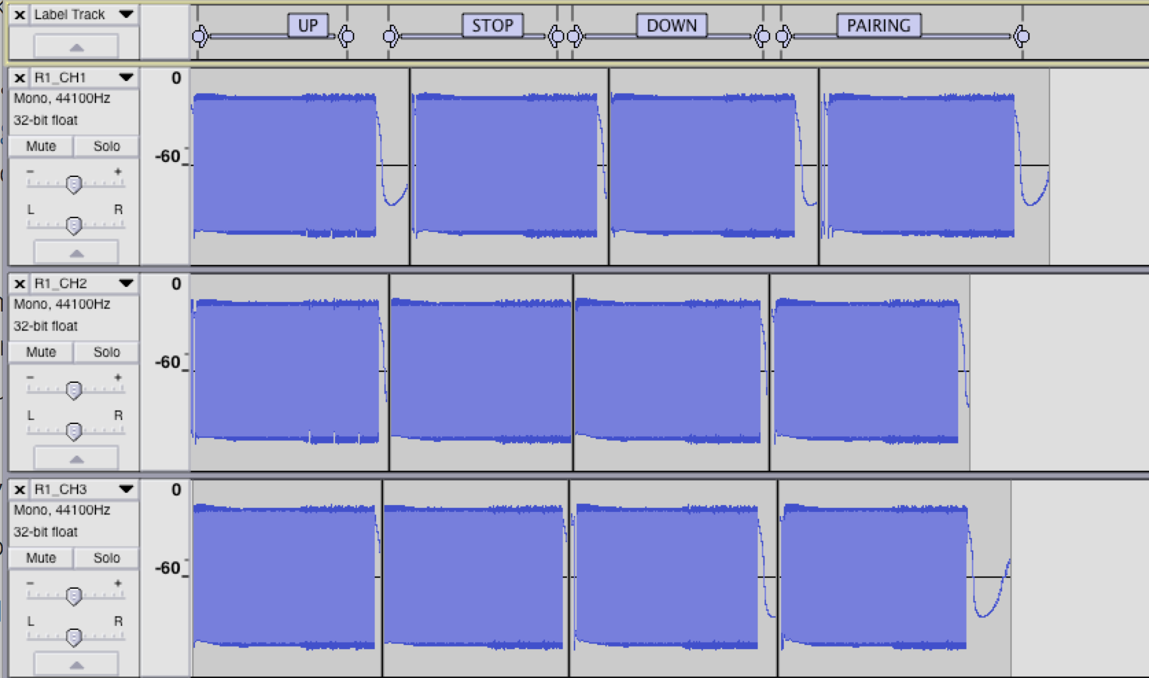
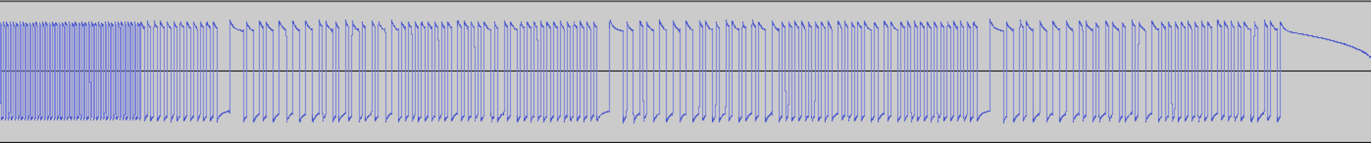
Zooming into the waveform, we can see the different parts of a captured transmission. This example below is the capture of Remote 1, Channel 1, for the pairing action:
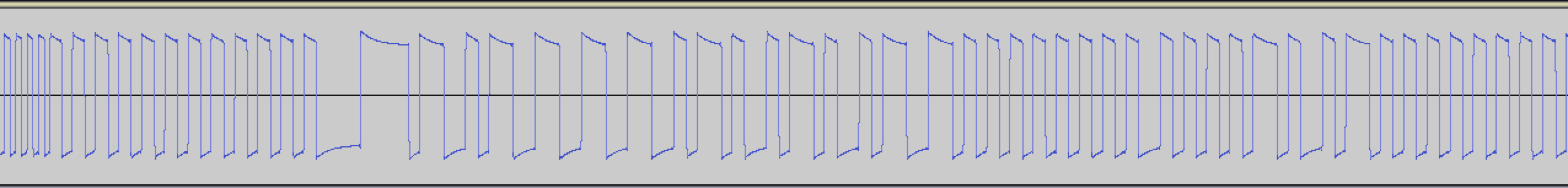
Zooming in:
In the zoomed image you can see that the transmission begins with a oscillating 0101 AGC pattern, followed by a further double width preamble pattern, followed by a longer header pattern, and then by data.
This preamble, header and data is repeated 3 times for R type remotes (The AGC pattern is only sent once at the beginning of transmission). This can be seen in the first image.
Looking at this data won’t be too useful. I need a way to turn it digital and analyse the bits and determine some patterns between different remotes, channels and actions.
Decoding the waveform.
We need to determine how the waveform is encoded. It’s very common for these kinds of hardware applications to use one of the following:
Raw? high long = 11, high short = 1, low long = 00, low short = 0?
By doing some research, I was able to determine that the encoding used was most likely manchester encoding. Let’s keep this in mind for later.
Digitising the data
I began processing the data as the raw scheme outlined above (even though I believed it was manchester). The reason for this is that if it happened to not be manchester, I could try decode it again with another scheme. (Also writing out raw by hand was easier than doing manchester decoding in my head).
I wrote out each capture into a Google Sheets spreadsheet. It took about 5 minutes to write out each action for each channel, and there were 6 channels per remote. I began to think this would take a while to actually get enough data to analyse. (Considering I had 160 captures to digitise)
I stopped once I collected all actions from 8 different channels across 2 remotes. This gave me 32 captures to play with. From this much data, I was able to infer a few things about the raw bits:
Some bits changed per channel
Some bits changed per remote.
Some bits changed seemingly randomly for each channel/remote/action combination.
Could this be some sort of checksum?
I still needed more data, but I had way too many captures to decode by hand. In order to get anywhere with this, I needed a script to process WAV files I captured via Audacity. I wrote a script that detected headers and extracted data as its raw encoding equivalent (as I had been doing by hand). This script produced output in JSON so I could add additional metadata and cross-check the captures with the waveform:
Once verified, I tabulated this data and inserted it into my spreadsheet for further processing. Unfortunately there was too many bits per capture to keep myself sane:
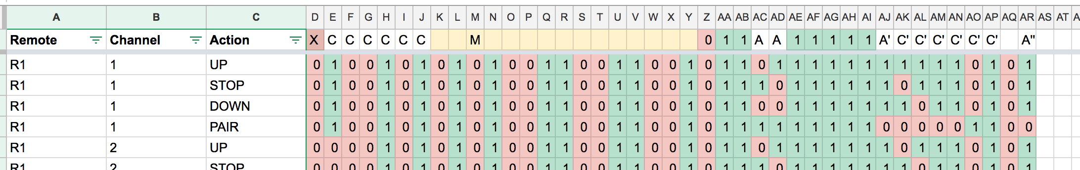
I decided it would be best if I decoded this as manchester. To do this, I wrote a script that processes the raw capture data into manchester (or other encoding types). Migrating this data into my spreadsheet, it begins to make a lot more sense.
Looking at this data we can immediately see some relationship between the bits and their purpose:
6 bits for channel (C)
2 bits for action (A)
6 bits for some checksum, appears to be a function of action and channel. F(A, C)
Changes when action changes
Changes when channel changes.
Cannot be certain it changes across remotes, since no channels are equal.
1 bit appears to be a function of Action F(A)
1 bit appears to be a function of F(A), thus, G(F(A)). It changes depending on F(A)’s value, sometimes 1-1 mapping, sometimes inverse mapping.
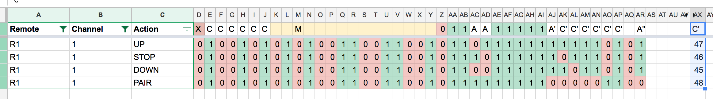
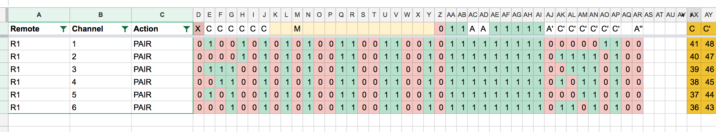
After some further investigation, I determined that for the same remote and channel, for each different action, the F(A, C) increased by 1. (if you consider the bits to be big-endian.).
Looking a bit more into this, I also determined that for adjacent channels, the bits associated with C (Channel) count upwards/backwards (X type remotes count upwards, R type remotes count backward). Additionally F(C) also increases/decreases together. Pay attention to the C column.
From this, I can confirm a relationship between F(A, C) and C, such that F(A, C) = F(PAIR, C0) == F(PAIR, C1) ± 1. After this discovery, I also determine that there’s another mathematical relationship between F(A, C) and A (Action).
Making More Data
From the information we’ve now gathered, it seems plausible that we can create new remotes by changing 6 bits of channel data, and mutating the checksum accordingly, following the mathematical relationship we found above. This means we can generate 64 channels from a single seed channel. This many channels is enough to control all the blinds in the house, however I really wanted to fully decode the checksum field and in turn, be able to generate an (almost) infinite amount of remotes.
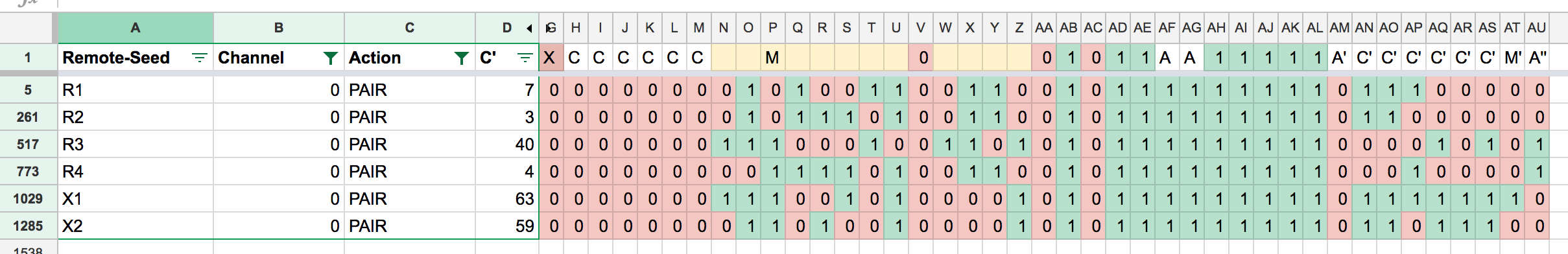
I wrote a tool to output all channels for a seed capture:
My reasoning behind generating more data was that maybe we could determine how the checksum is formed if we can view different remotes on the same channel. I.e. R0CH0, R1CH0, X1CH0, etc…
Essentially what I wanted to do was solve the following equation’s function G:
F(ACTION_PAIR, CH0) == G(F(ACTION_PAIR, CH0))
However, looking at all Channel 0’s PAIR captures, the checksum still appeared to be totally jumbled/random:
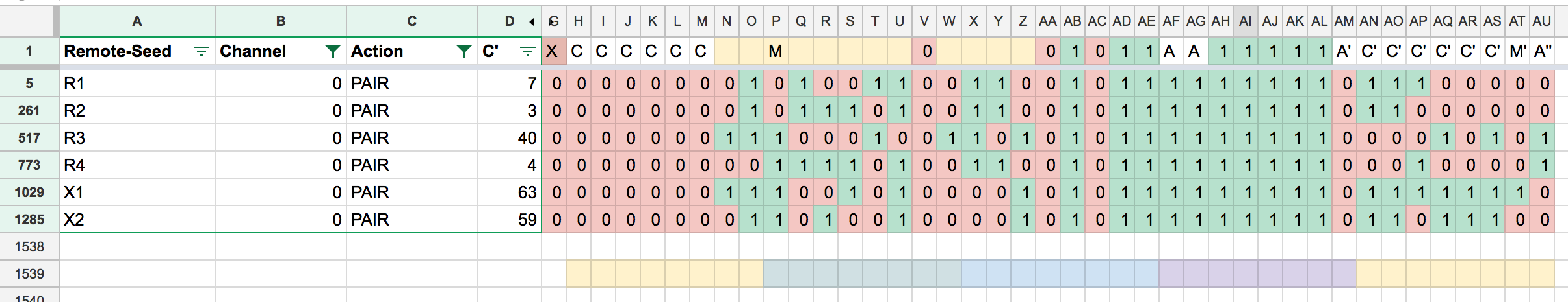
Whilst looking at this data, however, another pattern stands out. G(F(A)) sits an entire byte offset (8 bits) away from F(A). Additionally the first 2 bits of F(A, C) sit at the byte boundary and also align with A (Action). As Action increases, so does F(A, C). Lets line up all the bits at their byte boundaries and see what prevails:
Colours denoting byte boundaries
Aligned boundaries
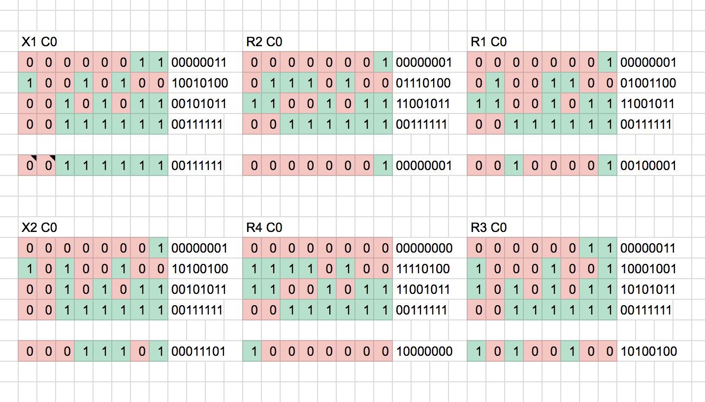
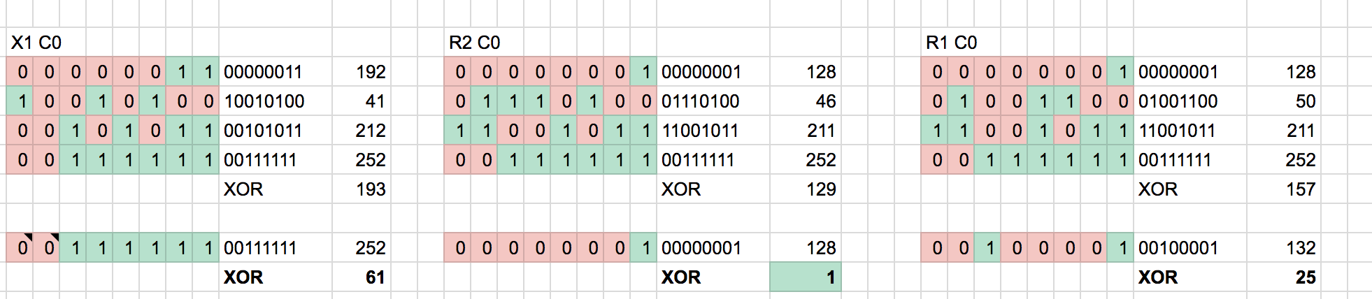
From here, we need to determine some function that produces the known checksum based on the first 4 bytes. Initially I try to do XOR across the bytes:
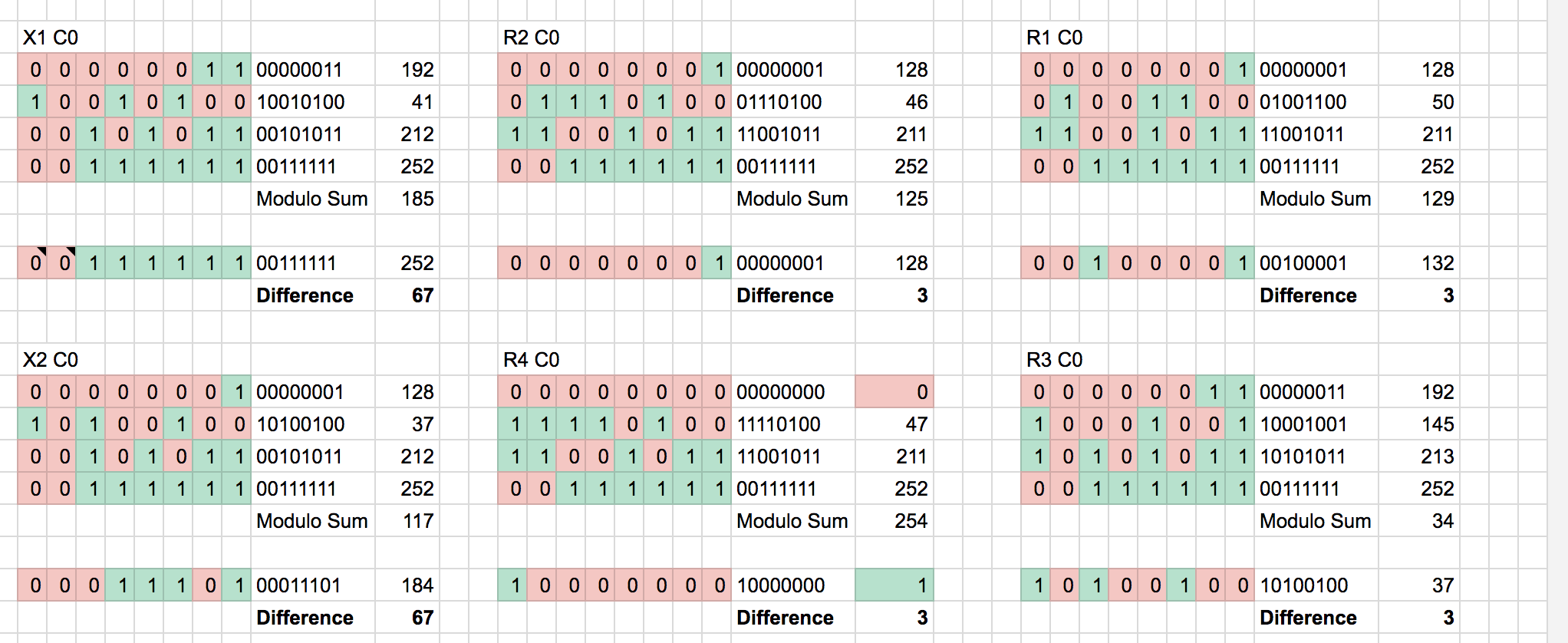
Not so successful. The output appears random and XOR’ing the output with the checksum does not produce a constant key. Therefore, I deduce the checksum isn’t produced via XOR. How about mathematical addition? We’ve already seen some addition/subtraction relationship above.
This appeared to be more promising - there was a constant difference between channels for identical type remotes. Could this constant be different across different type remotes because my generation program had a bug? Were we not wrapping the correct number of bits or using the wrong byte boundaries when mutating the channel or checksum?
It turns out that this was the reason 😑.
Solving the Checksum
Looking at the original captures, and performing the same modulo additions, we determine the checksum is computed by adding the leading 4 bytes and adding 3. I can’t determine why a 3 is used here, other than RAEX wanting to make decoding their checksum more difficult or to ensure a correct transmission pattern.
I refactored my application to handle the boundaries we had just identified:
typeRemoteCodestruct{LeadingBituint// Single bitChanneluint8Remoteuint16Actionuint8Checksumuint8}
Looking at the data like this began to make more sense. It turns out that F(A) wasn’t a function of A (Action), it was actually part of the action data being transmitted:
Additionally, the fact there is a split between channel and remote probably isn’t necessary. Instead this could just be an arbitrary 24 bit integer, however it is easier to work with splitting it up as an 8 bit int and a 16 bit int. Based on this, I can deduce that the protocol has room for 2^24 remotes (~16.7 million)! That’s a lot of blinds!
My remote-gen program was good for the purpose of generating codes using a seed remote (although, incorrect due to wrapping issues), however it now needed some additional functionality.
I needed a way to extract information from the captures and verify that all their checksums align with our rule-set for generating checksums. I wrote an info command:
Running with --validate exits with an error if the guessed checksum != checksum. Running this across all of our captures proved that our checksum function was correct.
Another piece of functionality the tool needed was the ability to generate arbitrary codes to create our own remotes:
./remote-gen create --channel=196 --remote=54654 --verbose
00010001101111110101010111111111010011001    Action: PAIR
00010001101111110101010110011111101101000    Action: DOWN
00010001101111110101010111011111111101000    Action: STOP
00010001101111110101010110111111100011000    Action: UP
I now can generate any remote I deem necessary using this tool.
Wrapping Up
There you have it, that’s how I reverse engineered an unknown protocol. I plan to follow up this post with some additional home-automation oriented blog posts in the future.
From here I’m going to need to build my transmitter to transmit my new, generated codes and build an interface into homekit for this via my homebridge program.
As mentioned above, if you are based in Australia, you can purchase these blinds and associated accessories in bulk or individually via www.raexaustralia.com (Full disclosure – my father runs the site)
Results are collected, optimised, and processed multiple times per day. Instagram images tagged with #hottest100 and a few others are included for counting.
Happy voting!
You can read about the process last year here. However, vote collection is a fair bit more accurate this year.
As a casual bike rider, I enjoy tracking my rides with Strava
so I can take a look at how my ride went and how well I performed throughout.
However, very rarely the Strava tracking application randomly
crashes, or gets killed by iOS on my phone, during the ride. This means
that the data was never recorded between the point at which the app died and
the point when I became aware the app had died.
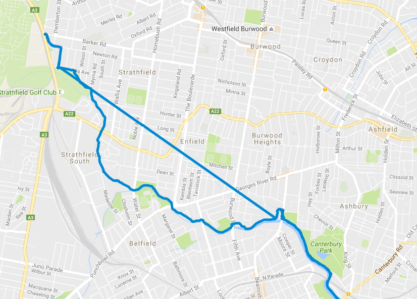
If we plot this type of failure, it looks something like this:
Fortunately in this case, there wasn’t too much missing data. However, I was
still determined to learn about the GPX format and see if I could patch up the
GPX file programatically.
In the specific case of the above map, I was riding north west, and at a point
Strava crashed. Between this point and when I pulled out my phone to check my
progress, no points were plotted. Google maps interprets this lack of data as
a straight line between to the 2 points (as per GPX specification).
If we crack open the GPX file and take a look, we can see exactly what this looks
like:
In it’s simplest form, a GPX file is an XML document that contains a sequence
of GPS points (with associated metadata like elevation, and other depending
on the tracker). This makes it reasonably simple for us to get our hands
dirty and begin fixing the data set.
In order to add the missing data back into the GPX file, we need 3 things:
The last coordinate recorded before the app crashed
The coordinate when the app was revived
A list of points of the track we want to use for our data points.
Fortunately, I was able to obtain a list of coordinates for the missing data
since I travelled the same path on the return journey (As can be seen on the
map above).
The other 2 app state points of interest are reasonably easy to find - just
find 2 data points that have a (reasonably) large time distance between them.
In order to process the data, I used a python library called gpxpy which
provided some good utilities for reading and processing a GPX file.
With this library, I was able to find the crash point, the revival point, and
the list of the points of the track. With this data, I interpolated the start/end
times of the crash points onto the track data, and spliced it back into the
dataset.
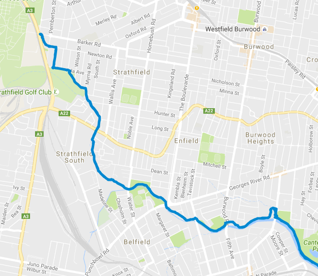
After exporting the data set, we achieve a map that looks like:
Quite clearly, this has a few limitations, for example, the calculated velocity
through all of the data points is simply an average. However, this did provide
me with an improved dataset which I could re-upload to Strava.
You can find all the source for this script
on my github


